3.7. SNA on Humanities Data: Creating the Graph

Now that we have created our node data and edge data, let’s go ahead and load them via Pandas.

import pandas as pd

nodes_df = pd.read_csv("../data/nodes.csv")
edges_df = pd.read_csv("../data/edges.csv")

nodes_df.head(1)

	name	color	place
0	0_Thabo Simon AARON	green	Bethulie

edges_df.head(1)

	source	target	place
0	ANC	0_Thabo Simon AARON	Bethulie

With this data, we can now construct a node list and edge list with just a few lines of Python. In the code below, we will be iterating over each DataFrame and creating lists of nodes and lists of edges sin the format that NetworkX expects. Remember, NetworkX wants to see each node in a node list rendered like this:

(NODE_ID, {METADATA})

Each edge in the edge list should be rendered like this:

(EDGE_SOURCE, EDGE_TARGET, {METADATA})

Remember, that these must be tuples and the meta data must be stored in the final index with each key being an attribute and each value being the value of that attribute.

nodes = []
edges = []
for idx, row in nodes_df.iterrows():
    nodes.append((row["name"], {"color": row.color, "place": row.place, "title": row["name"]}))
for idx, row in edges_df.iterrows():
    edges.append((row.source.strip(), row.target, {"place": row.place}))

nodes[0]

('0_Thabo Simon AARON',
 {'color': 'green', 'place': 'Bethulie', 'title': '0_Thabo Simon AARON'})

edges[0]

('ANC', '0_Thabo Simon AARON', {'place': 'Bethulie'})

3.7.1. Building the Network

from pyvis.network import Network
import networkx as nx

Now that we have our data structured correctly, we can begin constructing our network with NetworkX. We will first create our Graph class (G) and then add the nodes from our list of nodes and our edges from our list of edges.

G = nx.Graph()
G.add_nodes_from(nodes)
G.add_edges_from(edges)

When working with larger datasets, calculating the physics can often be time consuming when the PyVis HTML graph loads. For this reason, it can be useful to calculate the placement of the x and y coordinates beforehand. NetworkX gives us the ability to do this by leveraging the method of the algorithm we wish to use. In our case, we will use the spring_layout(). This method will take a single argument, the graph that we want to process. In our case, this is G.

This will return a list of lists. Each sublist will be x and y coordinates.

pos = nx.spring_layout(G)
pos['2_Nzaliseko Christopher ABRAHAM']

array([ 0.15706733, -0.01991105])

3.7.2. Visualizing the Network

First, we want to create our PyVis graph. We will be setting notebook to True because we are working within a Notebook.

net = Network(notebook=True)
net.from_nx(G)

Local cdn resources have problems on chrome/safari when used in jupyter-notebook. 

Let’s first take a look at the first node in our graph. We can access this individual’s node by grabbing index 0 in the nodes attribute of our net object.

net.nodes[0]

{'color': 'green',
 'place': 'Bethulie',
 'title': '0_Thabo Simon AARON',
 'size': 10,
 'id': '0_Thabo Simon AARON',
 'label': '0_Thabo Simon AARON',
 'shape': 'dot'}

Now we want this node to have an x and a y coordinate as attributes and we want this data to come from the pos object above which contains the data about each node’s position in the graph. To manually add these attributes to our nodes, we can use a for loop and create a new key of x and y and add those to each node.

for node in net.nodes:
    x, y = pos[node["id"]]
    node["x"] = x*10000
    node["y"] = y*10000

net.nodes[0]

{'color': 'green',
 'place': 'Bethulie',
 'title': '0_Thabo Simon AARON',
 'size': 10,
 'id': '0_Thabo Simon AARON',
 'label': '0_Thabo Simon AARON',
 'shape': 'dot',
 'x': 220.5653302371502,
 'y': 175.43811351060867}

Now that we have our PyVis graph created and assigned x and y coordinates, we can start to do some more advanced things. I can use get_adj_list() to create a dictionary of all nodes. Each key will be a unique node id. The values will be sets (lists with only unique items in each index) that correspond to the nodes to which they are connected. Because the purpose of this graph is to visualize relationships between people and organizations, set will include only organizations referenced in that individual’s description.

neighbor_map = net.get_adj_list()

neighbor_map["0_Thabo Simon AARON"]

{'ANC', 'ANCYL', 'Police', 'SAP'}

In the PyVis official documentation, this data is used to generate a title that will pop up when an individual hovers over it. It is modified slightly to replace the <br> HTML tag with \n.

for node in net.nodes:
    node["title"] += " Neighbors:\n" + "\n".join(neighbor_map[node["id"]])

net.nodes[0]

{'color': 'green',
 'place': 'Bethulie',
 'title': '0_Thabo Simon AARON Neighbors:\nSAP\nANCYL\nPolice\nANC',
 'size': 10,
 'id': '0_Thabo Simon AARON',
 'label': '0_Thabo Simon AARON',
 'shape': 'dot',
 'x': 220.5653302371502,
 'y': 175.43811351060867}

The number of connections in our graph also tells us the relative importance of a node. Remember, we have all individuals connected to organizations; we do not have individuals connected to other individuals. This means the organizations in our graph will have a larger number of connections. What if we wanted to use that information to increase the size of each node in the graph based on the number of unique connections? For this, we can set a node’s value based on the length of connections found in the neighbor_map.

for node in net.nodes:
    node["value"] = len(neighbor_map[node["id"]])

net.nodes[0]

{'color': 'green',
 'place': 'Bethulie',
 'title': '0_Thabo Simon AARON Neighbors:\nSAP\nANCYL\nPolice\nANC',
 'size': 10,
 'id': '0_Thabo Simon AARON',
 'label': '0_Thabo Simon AARON',
 'shape': 'dot',
 'x': 220.5653302371502,
 'y': 175.43811351060867,
 'value': 4}

Now that we have all of our data, we can now visualize it all. Because we already calculated the physics of our graph, we do not want to enable Physics, so we will set that to False.

net.toggle_physics(False)
net.save_graph("trc_graph.html")

The generated graph may be a bit difficult to interpret as the default window is quite zoomed out. This is because there are a lot of nodes in our graph that do not have any connections. A graph is a visual representation of mathematical relationships between nodes. The weaker nodes, or those with fewer connections, appear further away from the center of the graph. Likewise, stronger clusters, or those collection of nodes with the highest number of connections, will appear closer to the center. The gravity of these larger nodes push the smaller nodes with fewer connections further away in a spring loaded graph.

Because this is a dynamic graph, you can zoom in to examine the cluster if you are viewing this textbook online.

3.7.3. Adding Menus

Finding and isolating specific nodes in a large graph can be a bit difficult as well. What if you wanted to see where a specific node appeared? You would need to keep searching until you found that node. PyVis offers a solution to this problem with two types of menus. The first is a Select Menu. This allows you to select a specific node in the graph and highlight it. Depending on the graph size, it may take a few seconds for this visualization to take place. You can create a select menu with your graph by passing a keyword argument of select_menu and setting it to True when you first create your PyVis graph and call the Network class, like so:

net = Network(select_menu=True)

Note, if you are using a Jupyer Notebook to analyze your graph, this menu will appear but your graph data will not. This is due to the extra layer of JavaScript found within the HTML file. In order to visualize this graph, you will need to open it as a separate HTML file. The code below would create the same graph as above, but with a Select Menu.

net = Network(select_menu=True)
net.from_nx(G)
neighbor_map = net.get_adj_list()
for node in net.nodes:
    x, y = pos[node["id"]]
    node["x"] = x*10000
    node["y"] = y*10000
    node["title"] += " Neighbors:\n" + "\n".join(neighbor_map[node["id"]])
    node["value"] = len(neighbor_map[node["id"]])
net.toggle_physics(False)
net.save_graph("trc_graph_select.html")

When you open the generated HTML file, you will see this:

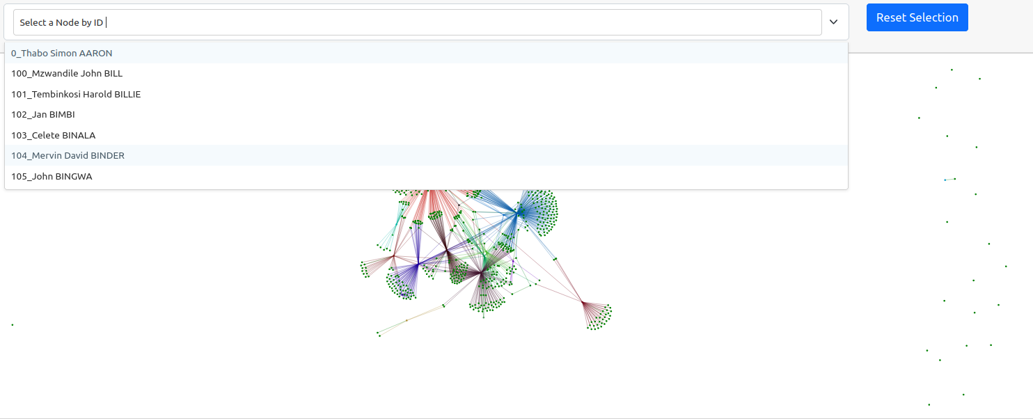
Fig. 3.1 Demonstration of Network Graph with a Select Menu

You can the select a node in the graph and highlight that particular node. Let’s say I wanted to see all nodes connected to the ANC in the graph. I would select ANC. The graph will then highlight that particular node and its connections.

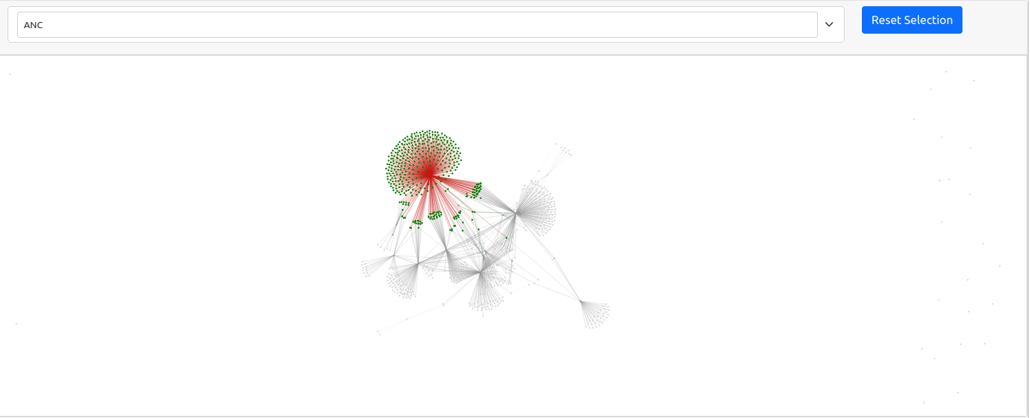
Fig. 3.2 Demonstration of Selecting Item in Select Menu

PyVis also offers a way to filter the graph with a Filter Menu. The filter menu allows you to find nodes or edges that have specific metadata. In the previous notebook, we made sure that our nodes and edges contained metadata about the place that was connected to it. This means that we can isolate the relevant edges or nodes in the graph with this metadata. Again, this makes it a lot easier to find relevant material and identify patterns in your data that may not be so easy to do as raw data. We can create a Filter Menu by passing a keyword argument filter_menu when we create the Network class and setting it to True.

net = Network(select_menu=True, filter_menu=True)
net.from_nx(G)
neighbor_map = net.get_adj_list()
for node in net.nodes:
    x, y = pos[node["id"]]
    node["x"] = x*10000
    node["y"] = y*10000
    node["title"] += " Neighbors:\n" + "\n".join(neighbor_map[node["id"]])
    node["value"] = len(neighbor_map[node["id"]])
net.toggle_physics(False)
net.save_graph("trc_graph_select_filter.html")

When you open the HTML file that is created, you will see the following graph:

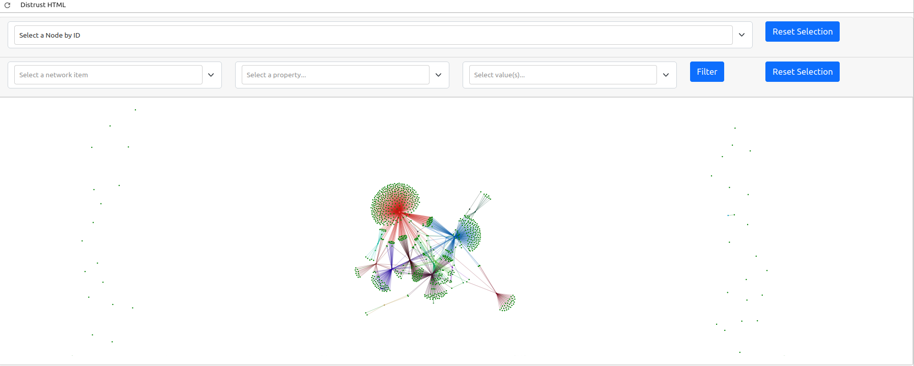
Fig. 3.3 Demonstration of Filter Menu in the Application.

Notice the addition of the Filter Menu below the Select Menu. You can select between nodes or edges as the item to filter and then select which piece of metadata. In our case, we want to filter by place. We then select the place that we want to isolate and view. In our case, let’s view Durban. We can then press Filter and view the results.

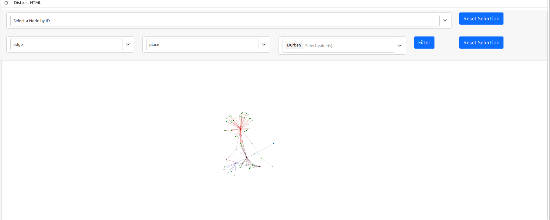
Fig. 3.4 Demonstration of Selecting Filters in the Filter Menu

3.7.4. Conclusion

Applying SNA to humanities data is not always the right solution to the problem, but if you are dealing with many pieces of data that are interconnected with different types of relationships, it can offer you a great way to quickly get a sense of patterns that you may otherwise miss. As a humanist, you can then use this information to generate questions or perhaps have a specific collection of sources or nodes that you can explore more closely. This chapter has not covered all aspects of SNA nor all the libraries for performing it via Python, but you should have a strong enough basis to begin applying it to your own data with minor modifications.